Introduction
Every year the Arctic Research Consortium of the US runs a competition to predict the mean arctic sea ice extent in September, and this year I have decided to enter. I have been an avid reader of Neven’s Arctic Sea Ice Blog for the last year, and they host predictions there too. The general idea is that in June, July and August a deadline is set for submissions of the prediction of the mean sea ice extent in September, using any methods available. One can submit as individuals or a team, professionally or personally. I thought I would put my modeling skills to the test, and see what I can do.
As background, arctic sea ice melts from May(ish) to September every year, reaching a minimum sometime in September, before the sun loses its strength and the whole area freezes up again. Over the past 20 years the melt has been strengthening, and recently extent and area have been in freefall. Records were broken in 2007 and then, spectacularly, again in 2012. Activity on Neven’s blog was frantic that year as the sea ice watchers tried to understand the enormity of the drop, and this year you can see again a whole bunch of very professional arctic observers watching the minutiae of the melting process. It’s fascinating because many of them are real experts in their field, and you can watch the joy of scientists learning new things about the world in real time, and see the enormous creativity they put into understanding the processes they are observing.
More seriously, arctic sea ice melt is expected to have significant effects on northern hemisphere weather, and understanding its accelerating destruction is important to understanding what is going to happen to northern hemisphere weather over the next 10-20 years. So, predictive modeling is not just a fun exercise, but a potentially useful tool to understand where the ice is going.
Method
[This is a relatively (for a stats methods section) tech-free methods, so you should be able to understand the gist without any prior education in statistics]
I used data on arctic sea ice extent and area from the National Snow and Ice Data Center (NSDIC), and northern hemisphere land-sea surface temperatures from the Goddard Institute for Space Studies (GISS, commonly called GISSTemp). I used the following variables to predict sea ice extent:
- Sea ice extent from the previous September
- May Extent, Area and northern hemisphere snow cover
- June Extent, area and northern hemisphere snow cover
- April and May surface temperature
June surface temperature was not available. Snow cover and surface temperatures are expressed as anomalies – the latter from the 1951 – 1980 baseline, the former from some baseline I can’t remember. I also used year in the model, since it’s reasonable to assume a trend over time.
I put all these variables into a Prais-Winsten regression model in Stata/MP 12. Prais-Winsten regression models enable multiple regression fitting of a single outcome variable to multiple predictors under the assumption of residuals with auto-correlation at lag 1, a common assumption that it is necessary to make in order to adjust for the serial dependence inherent in all time series. Since my main interest in this task is the point estimate (mean) of sea ice extent, I could have used a simple linear regression, but this would have given overly narrow confidence intervals. I could have looked for other modeling methods but Prais-Winsten is trivially easy in Stata, and I am lazy.
I didn’t use any model-building philosophy, just kept all variables in the model regardless of significance. I could have tried a couple of different models in competition, done some best-subset or backwards stepwise fitting, but given the amount of data I had (extent, area, snow cover and temperature readings for every month of the year) there was a big risk of over-fitting, so unless I crafted a careful ensemble model-fitting approach I risk producing a model that can explain everything and predict nothing. I have a day job, folks. So I just ran the one model. I may come back to the ensemble issue for the August estimate.
I first ran the model for the period 1979-2012 to check its fit and get parameter estimates. I then ran the model for the period 1979-2007, and obtained predicted values for 2008 – 2012. I did this to see if the model could accurately estimate the 2012 crash having only one prior major crash in the training data set. For the sake of interest, I then ran the model to 2011 and re-checked its predictive powers for 2012. Both are plotted in this report. I then ran the model to 2012 and used it to predict the mean September extent in 2013 with 95% prediction interval.
Results
The model converged and for the 1979-2012 period had an R-squared of 0.9303, indicating it explained 93% of the variance in the data. That’s quite ridiculous and highly suggestive of over-fitting. Table 1 contains the parameter estimates from this model.
Table 1: Parameter estimates from the full model (1979-2012)
| Variable |
Coefficient |
Standard Error |
T |
P value |
Lower CI |
Upper CI |
| Lagged Minimum Extent |
0.01 |
0.11 |
0.06 |
0.96 |
-0.22 |
0.24 |
| May Extent |
0.56 |
0.33 |
1.67 |
0.11 |
-0.13 |
1.25 |
| June Extent |
-1.04 |
0.41 |
-2.51 |
0.02 |
-1.89 |
-0.18 |
| May Area |
-0.91 |
0.46 |
-1.98 |
0.06 |
-1.85 |
0.04 |
| June Area |
1.85 |
0.32 |
5.75 |
0 |
1.18 |
2.51 |
| Year |
-0.07 |
0.02 |
-2.63 |
0.02 |
-0.12 |
-0.01 |
| June Snow Anomaly |
0.12 |
0.04 |
2.76 |
0.01 |
0.03 |
0.21 |
| April Temp |
-1.05 |
0.37 |
-2.85 |
0.01 |
-1.81 |
-0.29 |
| May Temp |
1.49 |
0.7 |
2.13 |
0.04 |
0.04 |
2.93 |
| Intercept |
136.22 |
51.41 |
2.65 |
0.01 |
29.88 |
242.57 |
These coefficients can be interpreted as indicating the amount by which the September mean extent varies in millions of kilometers for a unit change in the given value. So for example, every degree increase in April temperatures reduces the September extent by just over a million square kilometres, and there is a 70,000 square kilometer decline every year. Note the conflict between area and extent, and the strange protective effect of high temperatures in May. This is could be a sign of a model that is ignorant of physics, but just fits numbers to get the best fit. We probably shouldn’t try and use these coefficients to understand the physics of sea ice loss!
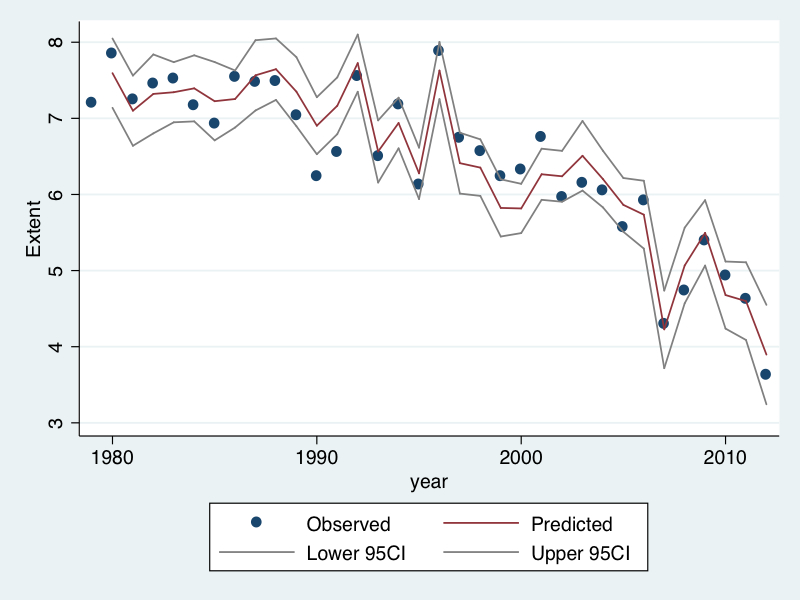
Figure 1 shows the predictive ability of the model run from 1979-2007. All values within this time frame are “within-sample” predictions, generally with low standard error and expected to be close to the true values. Values from 2008 – 2012 are “out of sample” predictions, with wider confidence intervals and greater risk of departure from the true value.

As can be seen, the model predicts the 2007 crash very well, but doesn’t handle the 2012 crash particularly brilliantly. It does predict a new record for 2012 though, guessing at a value of 4.13 million square kilometres, just below its 2007 estimate of 4.25. This is half a million square kilometres off the true value (3.63 million square kilometres).
Figure 2 shows the same fit for the same time periods when the model is run up to 2011. In this case only the year 2012 is an out-of-sample prediction.
This predictive fit is very good, estimating a value for 2012 of 3.90 million square kilometres – just 270,000 square kilometres off. Note that the 2012 true value is within the 95% confidence intervals for both predictive fits.
Using the model built for figure 2, I estimated the 2013 mean sea ice extent to be 4.69 million square kilometres, with 95% confidence interval 4.06 – 5.32 million square kilometres.
Conclusion
My final estimate for sea ice extent in September 2013 is 4.69 million square kilometres (95% CI: 4.06 – 5.32 million square kilometres). This is a huge recovery from September 2012, of just over 1 million square kilometres, but still historically a very low value. Given what I have read on the updates at Neven’s sea ice blog I find it hard to believe that this recovery could occur, but I also note that a lot of people are impressed by the slow early collapse of the ice, and think that unless the high summer is very unusual melting will be slower than last year. I also note that my model has successfully predicted the previous two crashes when run to one year before them, and doesn’t do a bad job of predicting crashes even five years out. I also note that in noisy series, data points don’t tend to continue below the trend for very long, so it’s about time for a correction. However, there is some concern that the persistent cyclone in May really destroyed a lot of ice and has prepared the arctic for a catastrophic summer.
Let’s hope my model is right!

Leave a comment