Recently I wrote a post criticizing an article at the National Bureau of Economic Research that found a legal ivory sale in 2008 led to an increase in elephant poaching. This paper used a measure of illegal poaching called commonly the PIKE, which is measured through counting carcasses discovered in searches of designated areas. This PIKE measures the proportion of deaths that are due to illegal poaching. I argued that the paper was wrong because the PIKE has a lot of zero or potentially missing values, and is bounded between 0 to 1 but the authors used ordinary least squares (OLS) regression to model this bounded number, which creates huge problems. As a result, I wasn’t convinced by their findings.
Since then I have read a few reports related to the problem. I downloaded the data and decided to have a look at an alternative, simple way of estimating the PIKE in which the estimate of the PIKE emerges naturally from a standard Poisson regression model of mortality. This analysis better handles the large number of zeros in the data, and also the non-linear nature of death counts. I estimated a very simple model, but I think a stronger model can be developed using all the standard properties of a well-designed Poisson regression model, rather than trying to massage a model misspecification with the wrong distributional assumptions to try and get the correct answer. This is an outline of my methods and results from the most basic model.
Methods
I obtained the data of legal and illegal elephant carcasses from the Monitoring Illegal Killing of Elephants (MIKE) website. This data indicates the region, country code, site number, and number of natural deaths and illegally killed elephants at each site in each year from 2002 – 2015. I used the full data set, although for comparing with the NBER paper I also used the 2003-2013 data only. I didn’t exclude any very large death numbers as the NBER authors did.
The data set contains a column for total deaths and a column for illegal deaths. I transformed the data into a data set with two records for each site-year, so that one row was illegal killings and one was total deaths. I then defined a covariate, we will call it X, that was 0 for illegal killings and 1 for total killings. We can then define a Poisson model as follows, where Y is the count of deaths in each row of the data set (each observation):
Y~Poisson(lambda) (1)
ln(lambda)=alpha+beta*X (2)
Here I have dropped various subscripts because I’m really bad at writing maths in wordpress, but there should be an i for each observation, obviously.
This simple model can appear confounding to people who’ve been raised on only OLS regression. It has two lines and no residuals, and it also introduces the quantity lambda and the natural logarithm, which in this case we call a link function. The twiddle in the first line indicates that Y is Poisson distributed. If you check the Poisson distribution entry in Wikipedia you will see that the parameter lambda gives the average of the distribution. In this case it measures the average number of deaths in the i-th row. When we solve the model, we use a method called maximum likelihood estimation to obtain the relationship between that average number of deaths and the parameters in the second line – but taking the natural log of that average first. The Poisson distribution is able to handle values of Y (observed deaths) that are 0, even though this average parameter lambda is not 0 – and the average parameter cannot be 0 for a Poisson distribution, which means the linear equation in the second line is always defined. If you look at the example probability distributions for the Poisson distribution at Wikipedia, you will note that for small values of lambda values of 0 and 1 are very common. The Poisson distribution is designed to handle data that gives large numbers of zeros, and carefully recalibrates the estimates of lambda to suit those zeros.
It’s not how Obama would do it, but it’s the correct method.
The value X has only two values in the basic model shown above: 0 for illegal deaths, and 1 for total deaths. When X=0 equation (2) becomes
ln(lambda)=alpha (3)
and when X=1 it becomes
ln(lambda)=alpha+beta (4)
But when X=0 the deaths are illegal; let’s denote these by lambda_ill. When X=1 we are looking at total deaths, which we denote lambda_tot. Then for X=1 we have
ln(lambda_tot)=alpha+beta
ln(lambda_tot)-alpha=beta
ln(lambda_tot)-ln(lambda_ill)=beta (5)
because from equation (3) we have alpha=ln(lambda_ill). Note that the average PIKE can be defined as
PIKE=lambda_ill/lambda_tot
Then, rearranging equation (5) slightly we have
ln(lambda_tot/lambda_ill)=beta
-ln(lambda_ill/lambda_tot)=beta
ln(PIKE)=-beta
So once we have used maximum likelihood estimation to solve for the value of beta, we can obtain
PIKE=exp(-beta)
as our estimate of the average PIKE, with confidence intervals.
Note that this estimate of PIKE wasn’t obtained directly by modeling it as data – it emerged organically through estimation of the average mortality counts. This method of estimating average mortality rates is absolutely 100% statistically robust, and so too is our estimate of PIKE, as it is simply an interpretation of a mathematical expression derived from a statistically robust estimation method.
We can expand this model to enable various additional estimations. We can add a time term to equation (2), but most importantly we can add a term for the ivory sale and its interaction with poaching type, which enables us to get an estimate of the effect of the sale on the average number of illegal deaths and an estimate of the effect of the sale on the average value of the PIKE. This is the model I fitted, including a time term. To estimate the basic values of the PIKE in each year I fitted a model with dummy variables for each year, the illegal/legal killing term (X) and no other terms. All models were fitted in Stata/MP 14.
Results
Figure 1 shows the average PIKE estimated from the mortality data with a simple model using dummy variables for each year and illegal/total killing term only.
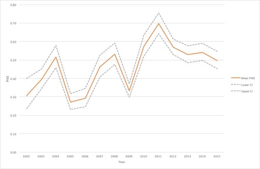
The average PIKE before the sale was 0.43 with 95% Confidence Interval (CI) 0.40 to 0.44. Average PIKE after increased by 26%, to 0.54 (95% CI: 0.52 to 056). This isn’t a very large increase, and it should be noted that the general theory is that poaching is unsustainable when the PIKE value exceeds 0.5. The nature of this small increase can be seen in Figure 2, which plots average total and illegal carcasses over time.
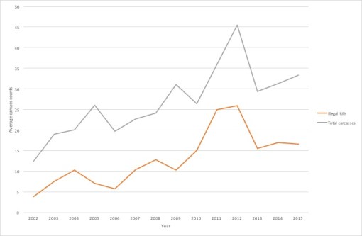
Although numbers of illegal carcasses increased over time, so did the number of legal carcasses. After adjusting for the time trend, illegal killings appear to have increased by a factor of 2.05 (95% CI 1.95 – 2.16) after the sale, and total kills by 1.58 (95% CI 1.53 – 1.64). Note that there appears to have been a big temporary spike in 2011-2012, but my results don’t change much if the data is analyzed from only 2003-2013.
Conclusion
Using a properly-specified model to estimate the PIKE as a side-effect of a basic model of average carcass counts, I found only a 25% increase in the PIKE despite very large increases in the number of illegal carcasses observed. This increase doesn’t appear to be just the effect of time, since after adjusting for time the post-2008 step is still significant, but there are a couple of possible explanations for it, including the drought effect mentioned by the authors of the NBER paper; some kind of relationship between illegal killing and overall mortality (for example because the oldest elephants are killed and this affects survival of the whole tribe); or an increase in monitoring activity. The baseline CITES report identified a relationship between the number of person-hours devoted to searching and the number of carcasses found, and the PIKE is significantly higher in areas with easy monitoring access. It’s also possible that it is related to elephant density.
I didn’t use exactly the same data as the NBER team for this model, so it may not be directly comparable – I built this model as an example of how to properly estimate the PIKE, not to get precise estimates of the PIKE. This model still has many flaws, and a better model would use the same structure but with the following adjustments:
- Random effects for site
- A random effect for country
- Incorporation of elephant populations, so that we are comparing rates rather than average carcasses. Population numbers are available in the baseline CITES report but I’m not sure if they’re still available
- Adjustment for age. Apparently baby elephant carcasses are hard to find but poachers only kill adults. Analyzing within age groups or adjusting for age might help to identify where the highest kill rates are and their possible effect on population models
- Adjustment for search effort and some other site-specific data (accessibility and size, perhaps)
- Addition of rhino data to enable a difference-in-difference analysis comparing with a population that wasn’t subject to the sale
These adjustments to the model would allow adjustment for the degree of searching and intervention involved in each country, which probably affect the ability to identify carcasses. It would also enable adjustment for possible contemporaneous changes in for example search effort. I don’t know how much of this data is available, but someone should use this model to estimate PIKE and changes in mortality rates using whatever is available.
Without the correct models, estimates of the PIKE and the associated implications are impossible. OLS models may be good enough for Obama, but they aren’t going to help any elephants. Through a properly constructed and adjusted Poisson regression model, we can get statistically robust estimates of the PIKE and trends in the PIKE, and we can better understand the real effect of interventions to control poaching.

Leave a comment