Compromise and Conceit

In comments to my post on balance in Shadowrun’s opposed skill checks, Paul asked me whether the distribution of success probabilities for opposed skill checks with equal numbers of dice is equal to the success probability you get from simply fixing an expected target number for your opponent. In practice what this means is that if the target number for success is, say, 5 or 6 on a d6 (probability 1/3) and both you and your opponent have, say, 6 dice, then you set an expected number of successes for your opponent as 6*1/3=2, and then try and roll over this expected target. Apparently Exalted 2e moved from challenged dice pools to using this process, fixing the target number to be half the opponent’s dice pool, and then having the attacker roll above it.

My guess in response was that this would be equivalent at larger dice pools. Turns out I was partially right and partially wrong. I ran a simulation in R, for dice pools from size 1 to 100, and set the target number of successes to be 1/3*(opponent’s dice pool), rounded down. So for a dice pool of 12, attacker rolls 12d6 and counts the number of successes (5 or 6s); they need to get over 12/3=4 to win. For 11 dice, the target is 11/3 rounded down, or 3. Figure 1 shows the results for opposed dice pools (black line) and the expected target number approach (red line).

Figure 1: Success probability with and without opposed dice pools

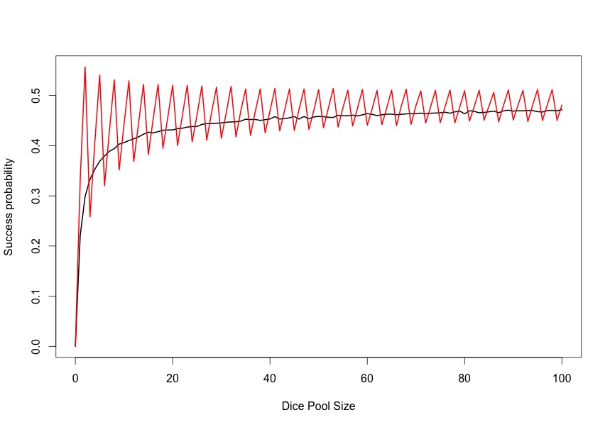
Note two interesting properties of this graph:

• The probability of success for the expected target approach bounces around a lot, going from above 0.5 to below 0.5 in little jagged steps. This is because of the rounding problem in setting expected targets. This means that even at large dice pools (100! imagine that!) you can still get large variations in success probability depending on whether your dice pool is a multiple of 3 or not
• The limiting value for opposed dice pools is not 0.5 as I thought, but actually closer to 0.47. I think this is because of the discrete nature of the probability distribution – there is a non-vanishing probability that both sides will roll the same number, whereas if the two dice pools were normally distributed this chance would be zero – someone always wins, and there is a 50% chance it will be you. In this case the normal approximation to the binomial distribution contains a small error even at dice pools of size 100 or more

The rounding problem is interesting because it is quite punishing at small dice pools. For example, if you have a dice pool of size 4 and your opponent also has size 4, then their expected target is rounded down to 1, which is actually the precise expected target for a dice pool of 3; you have actually gained a +1 to your dice pool through rounding error, and if your dice pools are both size 5 then this bonus increases to +2. We could use the opposite approach of rounding up, so then you would get a -1 or a -2 on your dice pool compared to your opponent. Rounding off smooths this problem a bit – in this case a target dice pool of size 4 gets an expected target of 1 (equivalent to 3d6); that of 5 gets an expected target of 2 (equivalent of 6d6). So your dice pool benefits or suffers. From the chart we can see that this effect is noticeable even at dice pools of 100d6 (which is why I extended it that far).

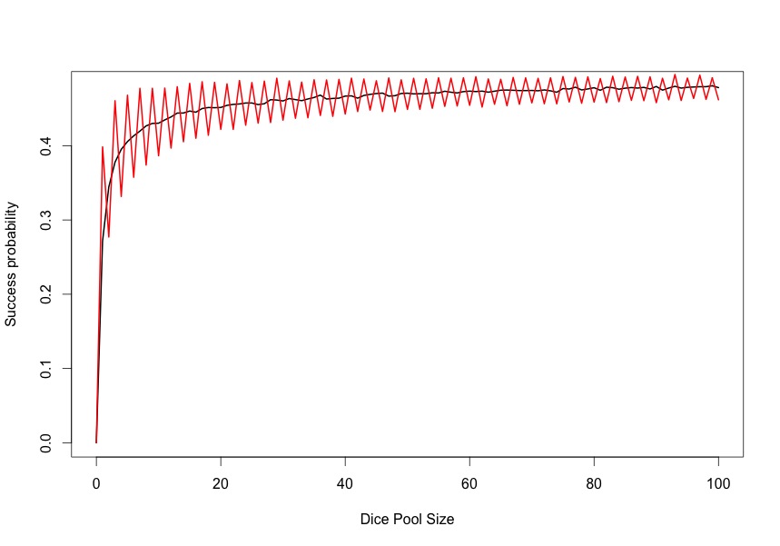
We can see more accurately what the true probability distributions would be like if we consider only dice pools that are multiples of 3 – that is dice pools of 3, 6, 12 etc. – because in this case there is no rounding error. This result is shown in figure 2, again with the opposed dice pool shown in black and the expected target number in red.

Figure 2: Results of dice pools with no rounding effect

Interestingly,with no rounding the expected target number method produces a slightly lower probability of success than the opposed dice pool method. This is because it restricts the range of extreme success available to the player – e.g. a player with a 6d6 pool can’t get success on a roll of 1 or 2 successes, even though this will (occasionally) happen.

I guess this means that the expected target number system is slightly broken, because rounding is very important at the scale of the dice pools that most people use. In the case of Shadowrun, for the first three dice pools (1d6 to 3d6) against a target with the same size dice pools, the probabilities of success are (respectively) 0.34, 0.56 and 0.26. So dice pools of 1 and 2 benefit hugely compared to dice pools of size 3. The same effect will exist in Exalted. What an expected target number system gains in simplicity, it loses in fairness (at least for small dice pools).

These kinds of considerations show that developing an effective system that is fun to use, simple and fair in all situations is fiendishly difficult. Next I am going to try and look at the WFRP 3 system to see if their methods based on opposed dice types are more robust to these kinds of concerns.

—

Update: Since Paul mentioned it in comments, Figure 3 shows an approximate example for Exalted 2e. It uses a target probability of 0.4 (7 or better on d10) but does not use exploding dice. The effect is still there but some of the jags are not as clear. Again, red line is the expected target number method, black line is the opposed check (so red=2e, black=1e?)

Figure 3: Target number vs. opposed check for Exalted dice pools

Update 2: apparently I got the dice pools wrong for Exalted, so I’ve updated Figure 3 using the correct numbers – a target probability of 0.5 and two successes on a roll of 10.